home |
copyright ©2019, tjmenzie@ncsu.edu

syllabus |
src |
submit |
chat
(Please note that this page uses materials from Joel Gruz's excellent book Data Mining from Scratch. Also, if there is anything missing from the following code, please see the raw source code. )
One of the most basic data mining algorithms is least squares regression. This algorithm tries to fit a straight line to a set of points. The best line is the one that reduces the square of the distance between the predicted and actual values.

LSR is described below, first in its simplest 2-dimensional form and then we handle the general N-dimensional case. When we get to the general case, a stochastic gradient descent (SDG) method will be used to optimize the β parameters of equations like y=α+β1x1+β2x2+β3x3+ ... (and in this case "optimize" means "guess β values in order to reduce the prediction errro". SDG is a perfect illustration of one of the main points of this book; i.e. that optimize and data mining and really very tightly connected.
First, we'll do the simple case
- Two-dimensional LSR (just
xversusy) - y= βx + α
Or, in Python
def predict(alpha, beta, x_i): return beta * x_i + alphaGiven a prediction y_i, then its error
and sum of errors squared is:
def error(alpha, beta, x_i, y_i):
  return y_i - predict(alpha, beta, x_i)

def sum_of_squared_errors(alpha, beta, x, y):
    return sum(error(alpha, beta, x_i, y_i) ** 2
               for x_i, y_i in zip(x, y))
The α and β terms can be computed from the standard deviation and correlation and covariance. Covariance is like a two-dimensional version of variance. Whereas variance measures how much values change from the mean, measures how two variables vary in tandem from their means.
def covariance(x, y):
  n = len(x)
  return dot(de_mean(x), de_mean(y)) / (n - 1)

def de_mean(x):
  """translate x by subtracting its mean
     (so the result has mean 0)"""
  x_bar = mean(x)
  return [x_i - x_bar for x_i in x]

def mean(x)          : return sum(x) / len(x)
def sum_of_squares(v): return dot(v, v)
def dot(v, w)        : return sum(v_i * w_i for v_i, w_i in zip(v, w))
Correlation is a number that varies
- -1 to 0 to 1 ;
- where -1 means perfectly linearly negatively associated;
- and 0 means no linear connection;
- and 1 means perfectly linearly positively associated.

def correlation(x, y):
  stdev_x = standard_deviation(x)
  stdev_y = standard_deviation(y)
  if stdev_x > 0 and stdev_y > 0:
    return covariance(x, y) / stdev_x / stdev_y
  else:
    return 0 # if no variation, correlation is zero

def standard_deviation(x):
  return math.sqrt(variance(x))

def variance(x):
  n = len(x)
  deviations = de_mean(x)
  return sum_of_squares(deviations) / (n - 1)
And finally:
def least_squares_fit(x,y):
  beta = correlation(x, y) * standard_deviation(y) / standard_deviation(x)
  alpha = mean(y) - beta * mean(x)
  return alpha, beta
For example:
num_friends = [ 100, 49, 41, 40, 25, 21, 21, 19, 19, 18, 18, 16,
15, 15, 15, 15, 14, 14, 13, 13, 13, 13, 12, 12, 11, 10, 10, 10, 10,
10, 10, 10, 10, 10, 10, 10, 10, 10, 10, 10, 9, 9, 9, 9, 9, 9, 9 ,
9, 9, 9, 9, 9, 9, 9, 9, 9, 9, 9, 8, 8, 8, 8, 8, 8, 8, 8, 8, 8, 8,
8, 8, 7, 7, 7, 7, 7, 7, 7, 7, 7, 7, 7, 7, 7, 7, 7, 6, 6, 6, 6, 6,
6, 6, 6, 6, 6, 6, 6, 6, 6, 6, 6, 6, 6, 6, 6, 6, 6, 5, 5, 5, 5, 5,
5 , 5, 5, 5, 5, 5, 5, 5, 5, 5, 4, 4, 4, 4, 4, 4, 4, 4, 4, 4, 4, 4,
4, 4, 4, 4, 4, 4, 4, 4, 3, 3, 3, 3, 3, 3, 3, 3, 3, 3, 3, 3, 3, 3,
3, 3, 3, 3, 3, 3, 2, 2, 2, 2, 2, 2, 2, 2, 2, 2, 2, 2, 2, 2, 2, 2,
2, 1, 1, 1, 1, 1, 1, 1, 1, 1, 1, 1, 1, 1, 1, 1, 1, 1, 1, 1, 1, 1,
1]

daily_minutes = [ 1, 68.77, 51.25, 52.08, 38.36, 44.54, 57.13, 51.4,
41.42, 31.22, 34.76, 54.01, 38.79, 47.59, 49.1, 27.66, 41.03, 36.73,
48.65, 28.12, 46.62, 35.57, 32.98, 35, 26.07, 23.77, 39.73, 40.57,
31.65, 31.21, 36.32, 20.45, 21.93, 26.02, 27.34, 23.49, 46.94, 30.5,
33.8,  24.23, 21.4, 27.94, 32.24, 40.57, 25.07, 19.42, 22.39, 18.42,
46.96, 23.72, 26.41, 26.97, 36.76, 40.32, 35.02, 29.47, 30.2, 31,
38.11, 38.18, 36.31, 21.03, 30.86, 36.07, 28.66, 29.08, 37.28,
15.28, 24.17, 22.31, 30.17, 25.53, 19.85, 35.37, 44.6, 17.23, 13.47,
26.33, 35.02, 32.09, 24.81, 19.33, 28.77, 24.26, 31.98, 25.73,
24.86, 16.28, 34.51, 15.23, 39.72, 40.8, 26.06, 35.76, 34.76, 16.13,
44.04, 18.03, 19.65, 32.62, 35.59, 39.43, 14.18, 35.24, 40.13,
41.82, 35.45, 36.07, 43.67, 24.61, 20.9, 21.9, 18.79, 27.61, 27.21,
26.61, 29.77, 20.59, 27.53, 13.82, 33.2, 25, 33.1, 36.65, 18.63,
14.87, 22.2, 36.81, 25.53, 24.62, 26.25, 18.21, 28.08, 19.42, 29.79,
32.8, 35.99, 28.32, 27.79, 35.88, 29.06, 36.28, 14.1, 36.63, 37.49,
26.9, 18.58, 38.48, 24.48, 18.95, 33.55, 14.24, 29.04, 32.51, 25.63,
22.22, 19, 32.73, 15.16, 13.9, 27.2, 32.01, 29.27, 33, 13.74, 20.42,
27.32, 18.23, 35.35, 28.48, 9.08, 24.62, 20.12, 35.26, 19.92, 31.02,
16.49, 12.16, 30.7, 31.22, 34.65, 13.13, 27.51, 33.2, 31.57, 14.1,
33.42, 17.44, 10.12, 24.42, 9.82, 23.39, 30.93, 15.03, 21.67, 31.09,
33.29, 22.61, 26.89, 23.48, 8.38, 27.81, 32.35, 23.84]

if __name__ == '__main__':
  print("variance(num_friends)", variance(num_friends))
  print("standard_deviation(num_friends)",
        standard_deviation(num_friends))
  print("covariance(num_friends, daily_minutes)",
        covariance(num_friends, daily_minutes))
  print("correlation(num_friends, daily_minutes)",
        correlation(num_friends, daily_minutes))
  print("alpha beta", least_squares_fit(num_friends, daily_minutes))
The output is:
variance(num_friends)	 81
standard_deviation(num_friends)	9.0
covariance(num_friends, daily_minutes)	22.425435139573054
correlation(num_friends, daily_minutes)	0.24819811705923378
alpha beta	(23.84486298346584, 0.8864062515241665)
That is, for the above data
- y = 0.88x + 23.8
- and the correlation is 0.25 (which is barely correlated at all).
To handle this, we need a vector for
the xs values and the
βs :
- [ α, β1x1, β2x2, β3x3, ]
which we can use in the following functions to find predictions, errors, and squared errors (in a manner similar to the above).
def predicts(x_i, beta)           : return dot(x_i, beta)
def errors(x_i, y_i, beta)        : return y_i - predicts(x_i, beta)
def squared_errors(x_i, y_i, beta): return errors(x_i, y_i, beta) ** 2
Then we do some gradient descent. This is like sking, when you are drunk. In this approach, to get to the bottom of a hill:
- Stand anywhere
- Lean over to every other point and write down the slope between you and them
- Move yourself along the average slope.
def estimate_beta(x, y):
    beta_initial = [random.random() for x_i in x[0]]
    return minimize_stochastic(squared_errors,
                               squared_error_gradients,
                               x, y,
                               beta_initial,
                               0.001)

def squared_error_gradients(x_i, y_i, beta):
    """the gradient corresponding to the ith squared error term.
       Derived via calculus applied to squared_errors."""
    return [-2 * x_ij * errors(x_i, y_i, beta)
            for x_ij in x_i]
For example:
# here are lots of examples of x1,x2,x3
xs = [[1,49,4,0],[1,41,9,0],[1,40,8,0],[1,25,6,0],[1,21,1,0],[1,21,0,0],[1,19,3,0],
      [1 ,19,0,0],[1,18,9,0],[1,18,8,0],[1,16,4,0],[1,15,3,0],[1,15,0,0],[1,15,2,0],
      [1,15,7,0],[1 ,14,0,0],[1,14,1,0],[1,13,1,0],[1,13,7,0],[1,13,4,0],[1,13,2,0],
      [1,12,5,0],[1,12,0,0],[1,11,9,0],[1,10,9,0],[1,10,1,0],[1,10,1,0],[1,10,7,0],
      [1,10,9,0],[1,10,1,0],[1,10,6,0],[1,10,6,0],[1,10,8,0],[1,10,10,0],[1,10,6,0],
      [1,10,0,0],[1,10,5,0],[1,10,3,0],[1,10,4,0],[1,9,9,0],[1,9,9,0],[1,9,0,0],
      [1,9,0,0],[1,9,6,0],[1,9,10,0],[1,9,8,0],[1,9,5,0],[1,9,2,0],[1,9,9,0],
      [1,9,10,0],[1,9,7,0],[1,9,2,0],[1,9,0,0],[1,9,4,0],[1,9,6,0],[1,9,4,0],
      [1,9,7,0],[1,8,3,0],[1,8,2,0],[1,8,4,0],[1,8,9,0],[1,8,2,0],[1,8,3,0],
      [1,8,5,0],[1,8,8,0],[1,8,0,0],[1,8,9,0],[1,8,10,0],[1,8,5,0],[1,8,5,0],
      [1,7,5,0],[1,7,5,0],[1,7,0,0],[1,7,2,0],[1,7,8,0],[1,7,10,0],[1,7,5,0],
      [1,7,3,0],[1,7,3,0],[1,7,6,0],[1,7,7,0],[1,7,7,0],[1,7,9,0],[1,7,3,0],
      [1,7,8,0],[1,6,4,0],[1,6,6,0],[1,6,4,0],[1,6,9,0],[1,6,0,0],[1,6,1,0],
      [1,6,4,0],[1,6,1,0],[1,6,0,0],[1,6,7,0],[1,6,0,0],[1,6,8,0],[1,6,4,0],
      [1,6,2,1],[1,6,1,1],[1,6,3,1],[1,6,6,1],[1,6,4,1],[1,6,4,1],[1,6,1,1],
      [1,6,3,1],[1,6,4,1],[1,5,1,1],[1,5,9,1],[1,5,4,1],[1,5,6,1],[1,5,4,1],
      [1,5,4,1],[1,5,10,1],[1,5,5,1],[1,5,2,1],[1,5,4,1],[1,5,4,1],[1,5,9,1],
      [1,5,3,1],[1,5,10,1],[1,5,2,1],[1,5,2,1],[1,5,9,1],[1,4,8,1],[1,4,6,1],
      [1,4,0,1],[1,4,10,1],[1,4,5,1],[1,4,10,1],[1,4,9,1],[1,4,1,1],[1,4,4,1],
      [1,4,4,1],[1,4,0,1],[1,4,3,1],[1,4,1,1],[1,4,3,1],[1,4,2,1],[1,4,4,1],
      [1,4,4,1],[1,4,8,1],[1,4,2,1],[1,4,4,1],[1,3,2,1],[1,3,6,1],[1,3,4,1],
      [1,3,7,1],[1,3,4,1],[1,3,1,1],[1,3,10,1],[1,3,3,1],[1,3,4,1],[1,3,7,1],
      [1,3,5,1],[1,3,6,1],[1,3,1,1],[1,3,6,1],[1,3,10,1],[1,3,2,1],[1,3,4,1],
      [1,3,2,1],[1,3,1,1],[1,3,5,1],[1,2,4,1],[1,2,2,1],[1,2,8,1],[1,2,3,1],
      [1,2,1,1],[1,2,9,1],[1,2,10,1],[1,2,9,1],[1,2,4,1],[1,2,5,1],[1,2,0,1],
      [1,2,9,1],[1,2,9,1],[1,2,0,1],[1,2,1,1],[1,2,1,1],[1,2,4,1],[1,1,0,1],
      [1,1,2,1],[1,1,2,1],[1,1,5,1],[1,1,3,1],[1,1,10,1],[1,1,6,1],[1,1,0,1],
      [1,1,8,1],[1,1,6,1],[1,1,4,1],[1,1,9,1],[1,1,9,1],[1,1,4,1],[1,1,2,1],
      [1,1,9,1],[1,1,0,1],[1,1,8,1],[1,1,6,1],[1,1,1,1],[1,1,1,1],[1,1,5,1]
      ]

# each i-th item from "ys" is the output see from the i-th input from "xs"

ys = [68.77, 51.25, 52.08, 38.36, 44.54, 57.13, 51.4, 41.42, 31.22,
34.76, 54.01, 38.79, 47.59, 49.1, 27.66, 41.03, 36.73, 48.65, 28.12,
46.62, 35.57, 32.98, 35, 26.07, 23.77, 39.73, 40.57, 31.65, 31.21,
36.32, 20.45, 21.93, 26.02, 27.34, 23.49, 46.94, 30.5, 33.8, 24.23,
21.4, 27.94, 32.24, 40.57, 25.07, 19.42, 22.39, 18.42, 46.96, 23.72,
26.41, 26.97, 36.76, 40.32, 35.02, 29.47, 30.2, 31, 38.11, 38.18,
36.31, 21.03, 30.86, 36.07, 28.66, 29.08, 37.28, 15.28, 24.17,
22.31, 30.17, 25.53, 19.85, 35.37, 44.6, 17.23, 13.47, 26.33, 35.02,
32.09, 24.81, 19.33, 28.77, 24.26, 31.98, 25.73, 24.86, 16.28,
34.51, 15.23, 39.72, 40.8, 26.06, 35.76, 34.76, 16.13, 44.04, 18.03,
19.65, 32.62, 35.59, 39.43, 14.18, 35.24, 40.13, 41.82, 35.45,
36.07, 43.67, 24.61, 20.9, 21.9, 18.79, 27.61, 27.21, 26.61, 29.77,
20.59, 27.53, 13.82, 33.2, 25, 33.1, 36.65, 18.63, 14.87, 22.2,
36.81, 25.53, 24.62, 26.25, 18.21, 28.08, 19.42, 29.79, 32.8, 35.99,
28.32, 27.79, 35.88, 29.06, 36.28, 14.1, 36.63, 37.49, 26.9, 18.58,
38.48, 24.48, 18.95, 33.55, 14.24, 29.04, 32.51, 25.63, 22.22, 19,
32.73, 15.16, 13.9, 27.2, 32.01, 29.27, 33, 13.74, 20.42, 27.32,
18.23, 35.35, 28.48, 9.08, 24.62, 20.12, 35.26, 19.92, 31.02, 16.49,
12.16, 30.7, 31.22, 34.65, 13.13, 27.51, 33.2, 31.57, 14.1, 33.42,
17.44, 10.12, 24.42, 9.82, 23.39, 30.93, 15.03, 21.67, 31.09, 33.29,
22.61, 26.89, 23.48, 8.38, 27.81, 32.35, 23.84]

random.seed(0)
beta= estimate_beta(xs,ys)
print(beta)
This prints
- [30.619881701311712, 0.9702056472470465, -1.8671913880379478, 0.9163711597955347]
- i.e. y= 30.62 + 0.97x1 - 1.87x2 + 0.92x3

- One thing to note about the following is that is shows an optimizer in the middle of a data miner.
- Another thing to note is that this optimizer makes many assumptions about the kind of function it is exploring.
- The benefit of making those assumptions is that, using those assumptions, certain calculations are fast to compute;
- But if the data does not correspond to those assumptions, then the resulting core fit will be very poor.
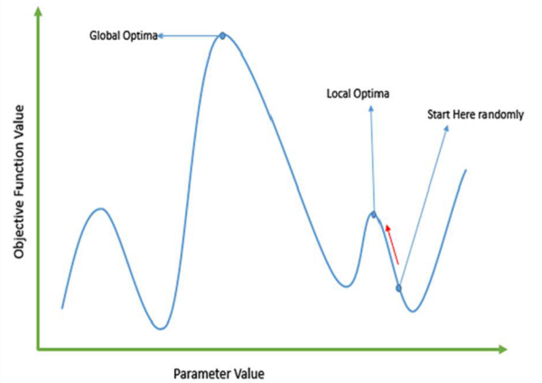
Also, gradient descent (gradient ascent) methods can get trapped by local optiima . In most real-world situations, we have many peaks and many valleys, which causes such methods to fail, as they suffer from an inherent tendency of getting stuck at the local optima:
Later in this book we will discuss optimizer that make far fewer assumptions about the function they are exploring.
def minimize_stochastic(target_fn, gradient_fn, x, y, theta_0, alpha_0=0.01):
    data = list(zip(x, y))
    theta = theta_0                             # initial guess
    alpha = alpha_0                             # initial step size
    min_theta, min_value = None, float("inf")   # the minimum so far
    iterations_with_no_improvement = 0
    # if we ever go 100 iterations with no improvement, stop
    while iterations_with_no_improvement < 100:
        value = sum( target_fn(x_i, y_i, theta) for x_i, y_i in data )
        if value < min_value:
            # if we've found a new minimum, remember it
            # and go back to the original step size
            min_theta, min_value = theta, value
            iterations_with_no_improvement = 0
            alpha = alpha_0
        else:
            # otherwise we're not improving, so try shrinking the step size
            iterations_with_no_improvement += 1
            alpha *= 0.9

        # and take a gradient step for each of the data points
        for x_i, y_i in in_random_order(data):
            gradient_i = gradient_fn(x_i, y_i, theta)
            theta = vector_subtract(theta, scalar_multiply(alpha, gradient_i))
    return min_theta

def squared_error(x_i, y_i, theta):
    alpha, beta = theta
    return error(alpha, beta, x_i, y_i) ** 2

def squared_error_gradient(x_i, y_i, theta):
    alpha, beta = theta
    return [-2 * error(alpha, beta, x_i, y_i),       # alpha partial derivative
            -2 * error(alpha, beta, x_i, y_i) * x_i] # beta partial derivative

def in_random_order(data):
    indexes = [i for i, _ in enumerate(data)]  # create a list of indexes
    random.shuffle(indexes)                    # shuffle them
    for i in indexes:                          # return the data in that order
        yield data[i]

def vector_subtract(v, w):
    return [v_i - w_i for v_i, w_i in zip(v,w)]

def scalar_multiply(c, v):
    return [c * v_i for v_i in v]