-
Notifications
You must be signed in to change notification settings - Fork 0
/
Copy path04b_dataspice.qmd
315 lines (201 loc) · 10.6 KB
/
04b_dataspice.qmd
1
2
3
4
5
6
7
8
9
10
11
12
13
14
15
16
17
18
19
20
21
22
23
24
25
26
27
28
29
30
31
32
33
34
35
36
37
38
39
40
41
42
43
44
45
46
47
48
49
50
51
52
53
54
55
56
57
58
59
60
61
62
63
64
65
66
67
68
69
70
71
72
73
74
75
76
77
78
79
80
81
82
83
84
85
86
87
88
89
90
91
92
93
94
95
96
97
98
99
100
101
102
103
104
105
106
107
108
109
110
111
112
113
114
115
116
117
118
119
120
121
122
123
124
125
126
127
128
129
130
131
132
133
134
135
136
137
138
139
140
141
142
143
144
145
146
147
148
149
150
151
152
153
154
155
156
157
158
159
160
161
162
163
164
165
166
167
168
169
170
171
172
173
174
175
176
177
178
179
180
181
182
183
184
185
186
187
188
189
190
191
192
193
194
195
196
197
198
199
200
201
202
203
204
205
206
207
208
209
210
211
212
213
214
215
216
217
218
219
220
221
222
223
224
225
226
227
228
229
230
231
232
233
234
235
236
237
238
239
240
241
242
243
244
245
246
247
248
249
250
251
252
253
254
255
256
257
258
259
260
261
262
263
264
265
266
267
268
269
270
271
272
273
274
275
276
277
278
279
280
281
282
283
284
285
286
287
288
289
290
291
292
293
294
295
296
297
298
299
300
301
302
303
304
305
306
307
308
309
310
311
312
313
314
315
---
title: "Creating metadata with `dataspice`"
subtitle: "Metadata"
---
The goal of this section is to provide a **practical exercise in creating metadata** for an **example field collected data product** using package `dataspice`.
- Understand basic metadata and why it is important.
- Understand where and how to store them.
- Understand how they can feed into more complex metadata objects.
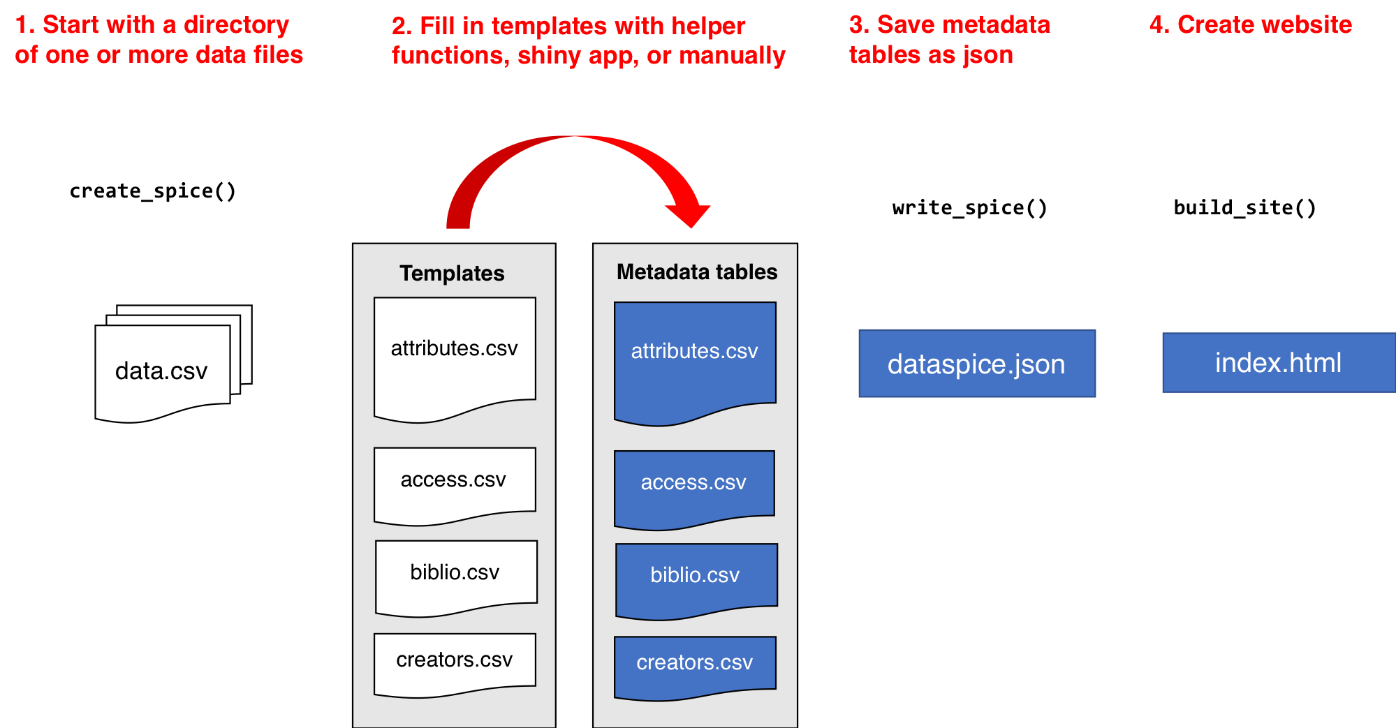
# `dataspice` workflow
*see [introductory slides](#04a_metadata_intro.qmd)*
Let's load our library and start creating some metadata! Let's also load `dplyr` which we'll use to extract and collect some metadata programmatically.
```{r}
#| message: false
library(dataspice)
library(dplyr)
```
# Create the metadata folder
We'll **start by creating the basic metadata `.csv` files** in which to collect metadata related to our example dataset using function **`dataspice::create_spice()`**.
```{r}
#| eval: false
create_spice()
```
This **creates a `metadata` folder** in your project's `data` folder (although you can specify a different directory if required) containing **4 `.csv` files** in which to record your metadata.

- **access.csv**: record details about where your data can be accessed.
- **attributes.csv**: record details about the variables in your data.
- **biblio.csv**: record dataset level metadata like title, description, licence and spatial and temoral coverage.
- **creators.csv**: record creator details.
# Record metadata
## `creators.csv`
> The `creators.csv` contains details of the **dataset creators**.
Let's start with a quick and easy file to complete, the **creators**. We can **open and edit** the file using in an **interactive shiny app** using **`dataspice::edit_creators()`**.
***Although we did not collect this data, just complete with your own details for the purposes of this tutorial.***
```{r}
#| eval: false
edit_creators()
```

Remember to click on **Save** when you're done editing.
<br>
## `access.csv`
> The `access.csv` contains details about **where the data can be accessed**.
Before manually completing any details in the `access.csv`, we can use `dataspice`'s dedicated function **`prep_access()` to extract relevant information** from the data files themselves.
```{r}
#| eval: false
prep_access()
```
Next, we can **use function `edit_access()`** to view `access`.
```{r, eval=FALSE}
edit_access()
```
The final details required, namely **the URL at which each dataset can be downloaded from** cannot be completed now so just leave that blank for now.
Eventually it should link to a permanent identifier from which the published. data set can be downloaded from.
We can also edit details such as the `name` field to something more informative if required.

Remember to click on **Save** when you're done editing.
<br>
## `biblio.csv`
> The `biblio.csv` contains dataset level metadata like **title**, **description**, **licence** and **spatial** and **temporal coverage**.
Before we start filling this table in, we can use some base R functions to extract some of the information we require. In particular we can **use function `range()` to extract the temporal and spatial extents of our data from the columns containing temporal and spatial data.**
Let's load our data.
```{r}
#| message: false
individual <- readr::read_csv(here::here("data", "individual.csv"))
```
### get **temporal extent**
Although dates are stored as a text string, **because they are in ISO format (YYYY-MM-DD), sorting them results in correct chronological ordering**. If your temporal data is not in ISO format, consider converting them (see package `lubridate`)
```{r}
range(individual$date)
```
### get **geographical extent**
The lat/lon coordinates are in decimal degrees which again are easy to sort or calculate the range in each dimension.
#### South/North boundaries
```{r}
range(individual$decimal_latitude)
```
#### West/East boundaries
```{r}
range(individual$decimal_longitude)
```
*NB: you can also supply the geographic boundaries of your data as a single [well-known text string](https://en.wikipedia.org/wiki/Well-known_text) in field `wktString` instead of supplying the four boundary coordinates.*
### Geographic description
We'll also need a geographic textual description.
Let's check the unique values in `domain_id` and use those to create a geographic description.
```{r}
unique(individual$domain_id)
```
We could use `NEON Domain areas D01:D09` for our geographic description.
Now that we've got the values for our temporal and spatial extents and decided on the geographic description, we can **complete the rest of the fields in the `biblio.csv` file using function `dataspice::edit_biblio()`**.
```{r, eval=FALSE}
edit_biblio()
```

::: {.alert .alert-success}
### :mag: metadata hunt
#### Complete the rest of the fields in `biblio.csv`
Additional information required to complete these fields can be found on the [**NEON data portal page for this dataset**](http://data.neonscience.org/data-product-view?dpCode=DP1.10098.001) and the **`data-raw/wood-survey-data-master`[README.md](data-raw/wood-survey-data-master/README.md)**
**Citation:** *National Ecological Observatory Network. 2020. Data Products: DP1.10098.001. Provisional data downloaded from http://data.neonscience.org on 2020-01-15. Battelle, Boulder, CO, USA*
Here's [an example to get you started](data/metadata/biblio-half.csv)
:::
Remember to click on **Save** when you're done editing.
<br>
## `attributes.csv`
> The `attributes.csv` contains details about the **variables** in your data.
Again, `dataspice` provides functionality to **populate the `attributes.csv` by extracting the variable names from our data file** using function **`dataspice::prep_attributes()`**.
The functions is vectorised and maps over each `.csv` file in our `data/` folder.
```{r, eval=FALSE}
prep_attributes()
```
```{r, out.width="100%", echo=FALSE}
knitr::include_graphics("assets/edit_attributes.png")
```
All column names in `individual.csv` have been successfully extracted into the `variableName` column.
Now, we could manually complete the `description` and `unitText` fields,... or we can use a secret weapon, `NEON_vst_variables.csv` in our raw data!
Let's read it in and have a look:
```{r}
variables <- readr::read_csv(here::here(
"data-raw", "wood-survey-data-master",
"NEON_vst_variables.csv"
))
variables
```
All original data variable names are contained in `fieldName`.
```{r}
variables$fieldName
```
Notice anything inconsistent with `variableName` in attributes? *hint: a hump*
Yes you guessed it, the original `fieldName`s are still in camelCase.
But! It also contains `description` and `units` columns! Just what we need!
::: {.alert .alert-success}
## Mega-Challenge!!
## Your challenge is to successfully merge the relevant contents of `variables` into our `attributes.csv`
You will need to save your merged table to `data/metadata/attributes.csv`.
Have a look at `janitor::make_clean_names()` and see if you can combine it with any other functions you've learned to mutate the values of columns to get round the camelCase names in `variables`. You'll need to have a good look at the `by` argument in the [`*_join` family](https://dplyr.tidyverse.org/reference/join.html) to figure out how to join by columns that contain the data you want to join by but have different names. You also will find `dplyr` function [`rename`](https://dplyr.tidyverse.org/reference/rename.html) useful!
Once you've completed your merge and saved it, use `dataspice::edit_attributes()` to fill in the final details for the few variables we created.
::: {.callout-tip appearance="minimal" collapse="true"}
# `dataspice` mega challenge solution
```{r}
variables <- readr::read_csv(
here::here(
"data-raw", "wood-survey-data-master",
"NEON_vst_variables.csv"
)
) %>%
dplyr::mutate(fieldName = janitor::make_clean_names(fieldName)) %>%
select(fieldName, description, units)
```
```{r, eval=FALSE}
attributes <- readr::read_csv(here::here("data", "metadata", "attributes.csv")) %>%
select(-description, -unitText)
```
```{r, echo=FALSE}
attributes <- readr::read_csv(here::here("data", "metadata", "attributes-prepped.csv")) %>%
select(-description, -unitText)
```
```{r echo=FALSE}
dplyr::left_join(attributes, variables, by = c("variableName" = "fieldName")) %>%
dplyr::rename(unitText = "units") %>%
readr::write_csv(here::here("data", "metadata", "attributes-complete.csv"))
```
```{r eval=FALSE}
dplyr::left_join(attributes, variables, by = c("variableName" = "fieldName")) %>%
dplyr::rename(unitText = "units") %>%
readr::write_csv(here::here("data", "metadata", "attributes.csv"))
```
:::
:::
# Create metadata json-ld file
Now that all our metadata files are complete, we can **compile it all into a structured `dataspice.json` file** in our `data/metadata/` folder.
```{r, eval=FALSE}
write_spice()
```
We can **read the `dataspice.json` file** into R as a list using the `jsonlite` function `read_json()` and then **inspect it using the `listviewer` package funtion `jsonedit`**.
```{r}
jsonlite::read_json(here::here("data", "metadata", "dataspice.json")) %>%
listviewer::jsonedit()
```
**Publishing this file on the web means it will be indexed by Google Datasets search!** :smiley: :+1:
<br>
------------------------------------------------------------------------
# Build README site
Finally, we can **use the `dataspice.json` file** we just created to **produce an informative README HTML web page** to include with our dataset for humans to enjoy! :star_struck:
We use function **`dataspice::build_site()`** which **creates file `index.html`** in the `data/` folder of your project (which it creates if it doesn't already exist).
```{r, eval=FALSE}
build_site(out_path = "data/index.html")
```
<br>
## View the resulting file [here](data/index.html)
<br>
Here's a screen shot!
```{r, out.width="100%", echo=FALSE}
knitr::include_graphics("assets/index_webshot.png")
```
## Example completed metadata files
- [`access.csv`](https://github.com/r-rse/rrresearch-acce-rrse/blob/main/data/metadata/access.csv)
- [`attributes.csv`](https://github.com/r-rse/rrresearch-acce-rrse/blob/main/data/metadata/attributes.csv)
- [`biblio.csv`](https://github.com/r-rse/rrresearch-acce-rrse/blob/main/data/metadata/biblio.csv)
- [`creators.csv`](https://github.com/r-rse/rrresearch-acce-rrse/blob/main/data/data/metadata/creators.csv)
------------------------------------------------------------------------
*back to the [outro slides](slides/04_metadata.html#30)*